About filter size

I recently got thinking about filter size. More specifically, I wondered whether we should use odd or even sized filter. One one hand, odd filter size seem more common and have easier interpretation (if the weight of the central pixel is far from 0). The interpretation is something along the line of take the central pixel and blend in information about its close neighbors. On the other hand, I’ve gotten much better results up to now with even sized filter. Also, it is pretty obvious that the filter size should depend on the input size as a 3×3 filter on a 128×128 image won’t capture the same level of details as a 3×3 filter on a 1024×1024 image. I don’t know that there are any rules to choosing filter sizes, but I will try and investigate further.

One thing I will implement (next week?) is multiple filter sizes in parallel as in Google’s Inception-3 model. This seems to be a best of both world solution and I hope it will improve my results.

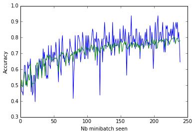
Accuracy graph for previous post

Here is the training graph for the NN described previously (which ends up with about 82% accuracy on test set after 5 epochs). Note that the train accuracy are calculated on a single mini-batch and the test accuracy are calculated on 10 times as many examples (except for end accuracy).

Follow up on class discussion

Today, we discussed a general rule to set the architecture of the last layer of a neural network. More specifically, we discussed how to set the output of a network and the loss of the network. Yoshua said that it is a good idea to have the network output a probability distribution over the r.v. Y (by either outputting a discrete distribution or the parameters of a continuous distribution) and the loss being -log P(Y=y|x) (the negative log-likelihood).

The problem I see with this is in the continuous case, since we are ditching the « non-parametricness » of the neural networks, which I find to be very desirable, by using (very often) multivariate normal distributions. I think so since, for one, their is a very small set of multivariate distributions from which to choose and most (not to say all) of those distributions are not very « complicated », for example, they have only one mode.

My first idea was to solve this by training a NN to output a NN that takes an input y (where y is in the domain of Y) and outputs P(Y=y|X=x) where x is the input to the first NN. But this seems overly complicated and possibly impossible to train. You would need to test tons of hyperparameters to get the size of the output NN to be good and I guess it would need to be fairly large because you aren’t passing expert knowledge to the network on what it is supposed to do. One would also need to make sure the output of the second NN is a distribution. One way to do it would be to integrate the output of the second NN, say z, over the domain of Y, to get say Z, and calculate the cost with z/Z. The integration should be pretty straight forward since we only have one input, one output and simple activation functions (ReLU are even piecewise linear) so we should be able to get a closed form expression.

My second idea is actually a cheat on the « parametricity ». There are some unidimensional distributions which can approximate any other distributions (for example, phase-type distribution for positive-valued distributions). The problem with these distributions is that they are often very hard to generalize to the multivariate case. One way to fix this would be to use copula to model the dependency between the various dimensions, but since copulas work on pairs of dimensions, it would be hard to use them.

It turns out, that there exist multivariate phase-type distributions! I didn’t know about them until now, but as I understand they are dense in the set of all positive-valued multivariate distributions. They can have has many parameters has we want depending on how good we want to approximate the complex distribution P(Y|X=x). The training would be a little bit fancy, but, if we chose a distribution which doesn’t have too many parameters, we might manage. I’d be very interested in trying something of the sort at some point. The obvious advantage would be that instead of only predicting a real valued output, we could calculate any quantities of interest, e.g. confidence intervals, variance, skewness, mode, median, …

I think it is not too far fetched to say that this neural network would need to output far less stuff than my first idea which required an output for every weight of the second NN. This is due to the fact that we are doing  mostly the same thing as in idea 1 except that we restrict the final function (our estimator for P(Y=y|X=x)) to be a distribution of a given type.

In most cases, maybe this extra information isn’t worth it, but I can see it being useful in various businesses. For example, in insurance, we would like to know, not only the average amount of losses a client might incur in the next year, but also how likely is he to cost more and what is the 99th quantile of his loss distribution and etc.

Psychology works!

So I must admit, I haven’t updated my blog and my repository as often as I should have. Still, my blog doesn’t reflect all the work I’ve done on the project! So in the next few days, I’m going to try and publish a few post showing the work I’ve done and what I’m hoping to achieve with the project.

The first entry in this serie (i.e. this post) will cover everything I’ve tried before hitting the 80% mark and maybe even more!

In my last post, I covered how I did my image preprocessing (still without data augmentation). Once that was setup, I went straight for the 80% goal! In hindsight, my first attempt was a bit overkill. I thought that I would make certain to get at least 80% accuracy by implementing a known network architecture, namely the VGG-16 (http://arxiv.org/abs/1409.1556).

I used Lasagne, to get everything in order fast and I trained my network from scratch. Without surprise, I got over 80% accuracy after a long training time. I didn’t save the training curves (maybe I will find time to run it again at some point to get them), since I don’t think this model is very interesting for the problem at hand.

Seeing how this model took about all the memory on my gpu even with small batch size, I got curious as to how small and simple could the model go and still hit the 80% mark. I inspired myself from Guillaume Alain’s model (https://gyomift6266h15.wordpress.com/2015/02/05/hit-the-80-mark-continued/) to get the following model (I’ll also update my github repo soon)

• Input is resized + cropped to 128×128 (I could probably even go smaller!)
• 32 filters convolution (4×4 filter)
• max pooling (2×2 window, 2×2 stride)
• 16 filters convolution (4×4 filter)
• max pooling (2×2 window, 2×2 stride)
• 16 filters convolution (4×4 filter)
• max pooling (2×2 window, 2×2 stride)
• 16 filters convolution (4×4 filter)
• max pooling (2×2 window, 2×2 stride)
• 16 filters convolution (4×4 filter)
• max pooling (2×2 window, 2×2 stride)
• 16 unit fully connected layer
• 16 unit fully connected layer
• 2 softmax unit

All non-linearities were ReLU. I used ADAM as my training algorithm. My batch size was set to 48…

And after as little as five epochs, my train and test errors were below 20%! I need to look into how to make training/test error plots, but for now here is my python console output :

 

# Neural Network with 24722 learnable parameters

## Layer information

# name size
— ——– ———-
0 input 3x128x128
1 conv2d1 32x125x125
2 maxpool1 32x62x62
3 conv2d2 16x59x59
4 maxpool2 16x29x29
5 conv2d3 16x26x26
6 maxpool3 16x13x13
7 conv2d4 16x10x10
8 maxpool4 16x5x5
9 dense1 16
10 dense2 16
11 output 2

[…]

sum(np.equal(y_test, preds))/len(preds)
Out: 0.8125

In my next post, I’ll probably cover what I’m looking at now, or what I want to try next. I should also do a post on the problems I encountered and how I fixed them.